Introduction

In this post we will be exploring and understanding one of the basic Classification Techniques in Machine Learning – Logistic Regression.

• Binary logistic regression: It has only two possible outcomes. Example- yes or no
• Multinomial logistic regression: It has three or more nominal categories. Example- cat, dog, elephant.
• Ordinal logistic regression– It has three or more ordinal categories, ordinal meaning that the categories will be in a order. Example- user ratings(1–5).

For now, lets focus on Binary Logistic Regression.

Logistic Regression

Logistic regression model is used to calculate predicted probabilities at specific values of a key predictor, usually when holding all other predictors constant.

Lets take the example of predicting if patient has 10-year risk of future coronary heart disease (CHD).

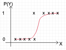
Possible predictors could be patient’s heart rate, BP, smoker/non-smoker etc. . We want to predict if the patient will has 10-year risk of future coronary heart disease (CHD) or not . We can have a decision boundary eg.: 0.5 such that P(Y) > 0.5 , classify patient as at risk and P(Y) < 0.5, classify patient as not at risk.

So basically, if a model has to succeed in predicting this, we need individual predictor (X) to have a constant effect on the probability of patient at risk of CHD [P(Y)]. But, the effect of X on the probability of Y has different values depending on the value of X.

This is where Odds come into picture as the odds ratio represent the constant effect of a predictor X on the likelihood that Y will occur.

Odds

Odds tell you the likelihood of an outcome. To those who are not familiar with the concept of Odds, here is an example.

Lets say Y represents the patients being at risk and Z represents the patients not being a risk, and someone says the odds of event Y is 1/3. Now what does that mean?

Out of 4 patients, 1 would be at risk and 3 would not be at risk.
So the Odds of patients being at risk are 1:3 .

That’s the difference between Probability and Odds. The probability in this case would be P(Y) = 1/(3+1) = 1/4.
Probability takes all outcomes into consideration (3 not at risk + 1 at risk).

Probability and Odds are related mathematically.

If P(Y) = probability of patient at risk , then 1-P(Y) would give the probability of patient not at risk

Logistic regression uses Sigmoid function to predict probability.

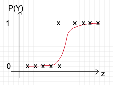
Equation for Sigmoid function : 1/(1+ e^-z), where

Now lets derive log(Odds) knowing P(Y) = 1/(1+ e^-z)

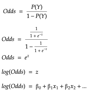
Here x₁ , x₂ .. represent the predictors and β₁ , β₂ … represent the constant effect of the predictors that we talked earlier.

Cost Function

Cost function basically quantifies the difference between models’ predicted values and actual values, giving you the error value.

Here we cant use the Cost function of Linear Regression (MSE), since h_θ(x) [sigmoid function] is non-linear function, using MSE would result in a non-convex function with many local minimums. Gradient Descent would not be able to find the global minimum successfully when many local minimums are present.

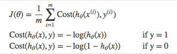
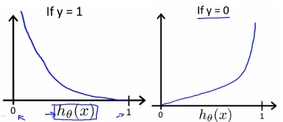
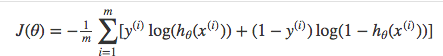
Above functions combined into one gives us the final cost function.

Logistic Regression using sklearn

sklearn has an implementation of Logistic Regression which makes it very easy on our part to just call the functions fit() and predict() to get the classifications done.

Lets take an example dataset of patients who have risk of getting CHD (coronary heart disease) in 10 years.

df = pd.read_csv("framingham.csv")
df.info()

print("Percentage of People with heart disease: {0:.2f} %".format(100*df.TenYearCHD.value_counts()[1]/df.TenYearCHD.count()))

Output: Percentage of People with heart disease: 15.23 %

After performing cleaning operations and weeding out statistically insignificant variables, let’s create new dataframe and perform logistic regression.

# Creating new dataframe with statistically significant columns
new_df=df[['male','age','cigsPerDay','prevalentHyp','diabetes','sysBP','diaBP','BMI','heartRate','ed__2.0','ed__3.0','ed__4.0', 'TenYearCHD']]

# Splitting into predictors and label
X = new_df.drop(['TenYearCHD'], axis=1)
Y = new_df.TenYearCHD

# Splitting dataset into train and test in the ratio 7:3
x_train,x_test,y_train,y_test = train_test_split(X,Y,test_size=0.3,random_state=5)

Now we’re all set to apply sklearn’s logistic regression functions

logreg = LogisticRegression()
logreg.fit(x_train,y_train)
y_pred = logreg.predict(x_test)

y_pred holds all the predicted values for dependent variable (TenYearCHD). Now let’s check the accuracy of the model.

sklearn.metrics.accuracy_score(y_test,y_pred)

Output: 0.860655737704918

This means that our model was able to correctly classify 86% of the test data which is a good number (whether this value is satisfactory or not depends on the business case). In case this isn’t satisfactory, there are optimization techniques to improve the model, or different classification techniques can be used, these will be discussed in coming posts.

The complete notebook for the above example can be found at Kaggle and Github.